L15 - Satellite System in Agriculture

Gustavo Alckmin

July 25, 2025

Satellite Data for Precision Agriculture

• Early precision farming relied on Landsat: 30 m spatial resolution, 15-day revisit, cloud interference
  
• Spatial layers fed prescription maps for variable-rate fertilization, pesticide, and tillage
  
• Baseline crop/soil status from surveys, field sampling, lab analysis plus point sensors
  
• Critical need for frequent, cost-effective, fine-scale spatial data over heterogeneous fields
  
• Emerging remote-sensing solutions: high-resolution satellites, hyperspectral, SAR
  • In WA: e.g., Sentinel-2 for reliable multispectral data, Sentinel-1 (SAR) for cloud penetration, and PlanetScope for high temporal resolution.
• Goal: real-time monitoring of crop nutrition, growth, yield, and soil properties
  • In WA: Tackling challenges like nutrient variability in sandy soils, and monitoring large-scale broadacre crops across the Wheatbelt.

Precision agriculture’s evolution hinged on the ability to map field variability. In the 1990s, Landsat’s 30 m ground sample distance and 15-day overpass, further hampered by cloud cover, constrained temporal and spatial resolution. Nevertheless, these images enabled the first generation of prescription maps driving variable-rate fertilizer, pesticide, and tillage regimes tailored to management zones. Traditional agronomic assessment—surveys, soil cores, lab analyses—provided static snapshots, now supplemented by ground-truth data from local bodies like DPIRD and GRDC through trial sites and soil moisture probe networks.

The real technical barrier remains acquiring high-resolution, revisit-frequent spatial data across large acreages at acceptable cost. Advances in small-satellite constellations (PlanetScope, Sentinel series), UAV-mounted multispectral and hyperspectral sensors, and SAR platforms now offer sub-meter resolution and daily to weekly coverage. Integrating these data streams supports dynamic tracking of crop nutrition, phenology, water stress, biomass, and soil moisture, informing precise, in-season variable-rate applications. Research confirms that finer spatial detail and shorter revisit intervals can improve input use efficiency, yield consistency, and environmental outcomes by enabling truly site-specific management.

Agenda

• Introduction to Remote Sensing Principles for WA Agriculture
• Key Satellite Platforms & Data Sources for the WA Wheatbelt (Sentinel, Landsat, PlanetScope)
• Application I: Mapping and Managing Soil
• Application II: In-Season Crop Monitoring (NDVI, NDRE) for Wheat & Canola
• Application III: Integrating SAR for Soil Moisture Estimation
• Data to Decision: Workflow from Satellite Imagery to VRT
• Future Trends: AI, Data Fusion, and UAV integration in WA

This slide outlines the key topics we will cover. First, we will examine recent advancements in precision agriculture and integrated pest management tools, referencing pivotal studies that provide both modeling frameworks and field-validated applications. Next, we introduce the cognitive model of decision-making in IPM, based on March (1994), which frames how choices are structured. We then break down the three hierarchical levels of decisions: - Strategic: long-range planning at farm or landscape scale, including crop rotation and cultivar selection to pre-empt disease (Conway 1984; McCown 2002; Rossi et al. 2012). - Tactical: short-term choices on when and which protection measures to use, optimizing interventions based on current crop and pest status. - Operational: real-time implementation and refinement of these tactics in response to evolving field conditions. Finally, we will transition into our detailed methodology and case studies to illustrate these concepts in action.

What is Remote Sensing?

• Definition: Non-contact measurement of Earth features across visible and nonvisible EM spectra
  
• Encompasses aerial, satellite, radar, and thermal instruments
  
• Proximal sensing vs. remote sensing distinctions
  
• Real-Time Kinematic (RTK) GPS for sub-cm geolocation
  
• Rate controllers link spatial data to variable-rate applications
• Applications in WA: e.g., mapping soil types in the Ord River Irrigation Area, monitoring canopy health (NDVI) in Margaret River vineyards, and delineating management zones in broadacre wheat fields.

graph LR
  A[Remote Sensing] --> B[Satellite Imagery]
  A --> C[Aerial Photography]
  A --> D[Radar]
  A --> E[Thermal Imaging]
  A --> F[Proximal Sensors]
  style A fill:#f9f,stroke:#333,stroke-width:1px

Remote sensing emerged in the late 1970s to describe Earth-observation beyond conventional aerial photography, extending into nonvisible wavelengths and spaceborne platforms. It refers to any measurement or information acquisition about a target without physical contact. This broad definition includes proximal sensors—devices placed near the target—and fully remote instruments on aircraft or satellites. Core technologies include color and color-infrared aerial photography, multispectral and hyperspectral satellite imagery, radar (e.g., SAR), and thermal imaging. RTK GPS enhances spatial accuracy by transmitting carrier-phase corrections from fixed reference stations to mobile units, a crucial component for controlled traffic farming (CTF) on large WA farms. In precision agriculture, remote sensing data feed rate controllers to apply inputs variably across fields. Key uses are early plant stress detection, mapping soil moisture and irrigation inefficiencies, distinguishing vegetation cover from bare soil, and defining management zones for site-specific treatments.

Electromagnetic Spectrum in Agriculture

• Ultraviolet (100–400 nm) through microwave (1 mm–1 m) spectral range used in PA operations
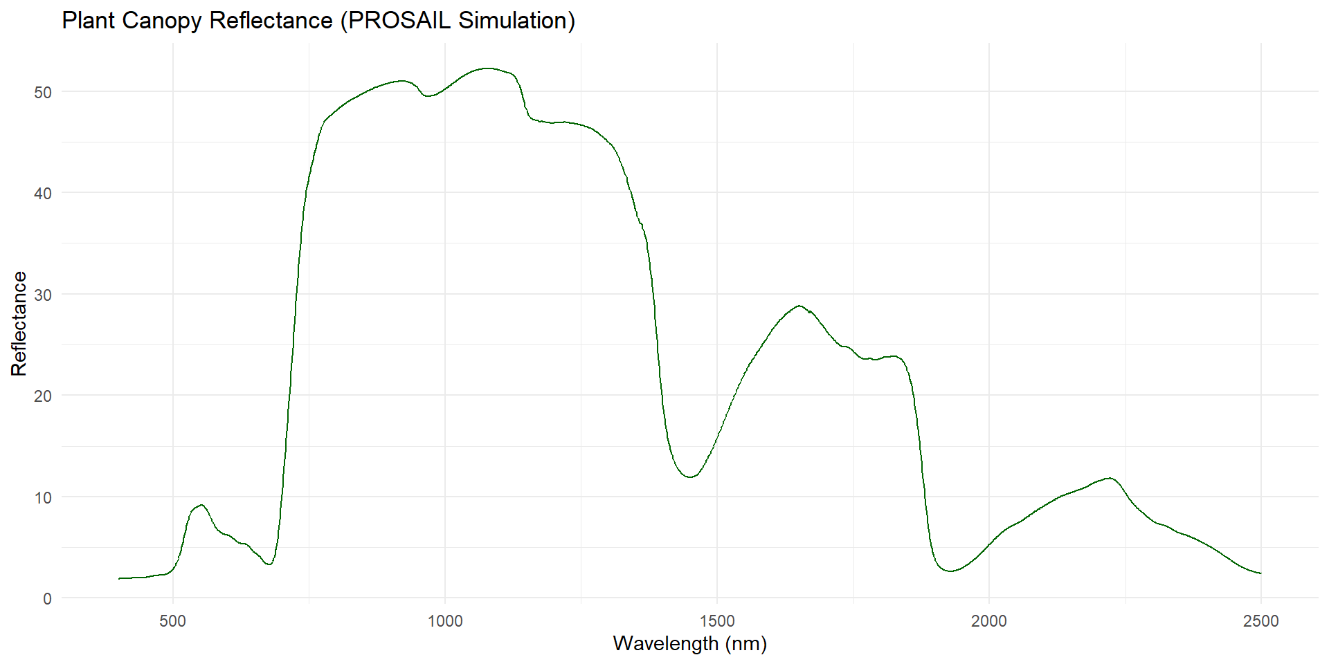
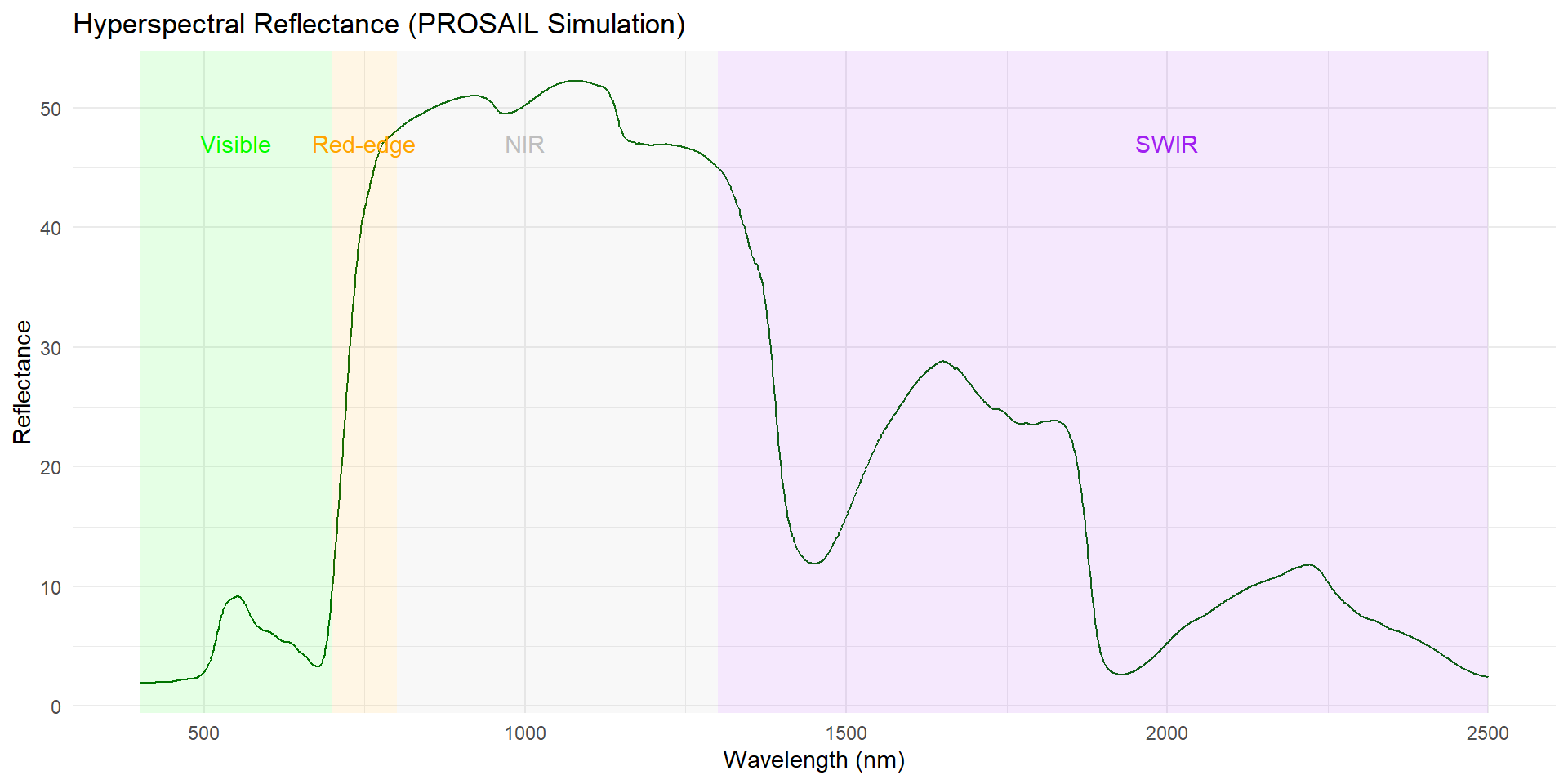
• Visible (400–700 nm) and NIR (700–1100 nm) bands for vegetation indices (e.g., NDVI, EVI)
• SWIR (Short-Wave Infrared) bands are critical in WA for assessing soil and crop moisture content.
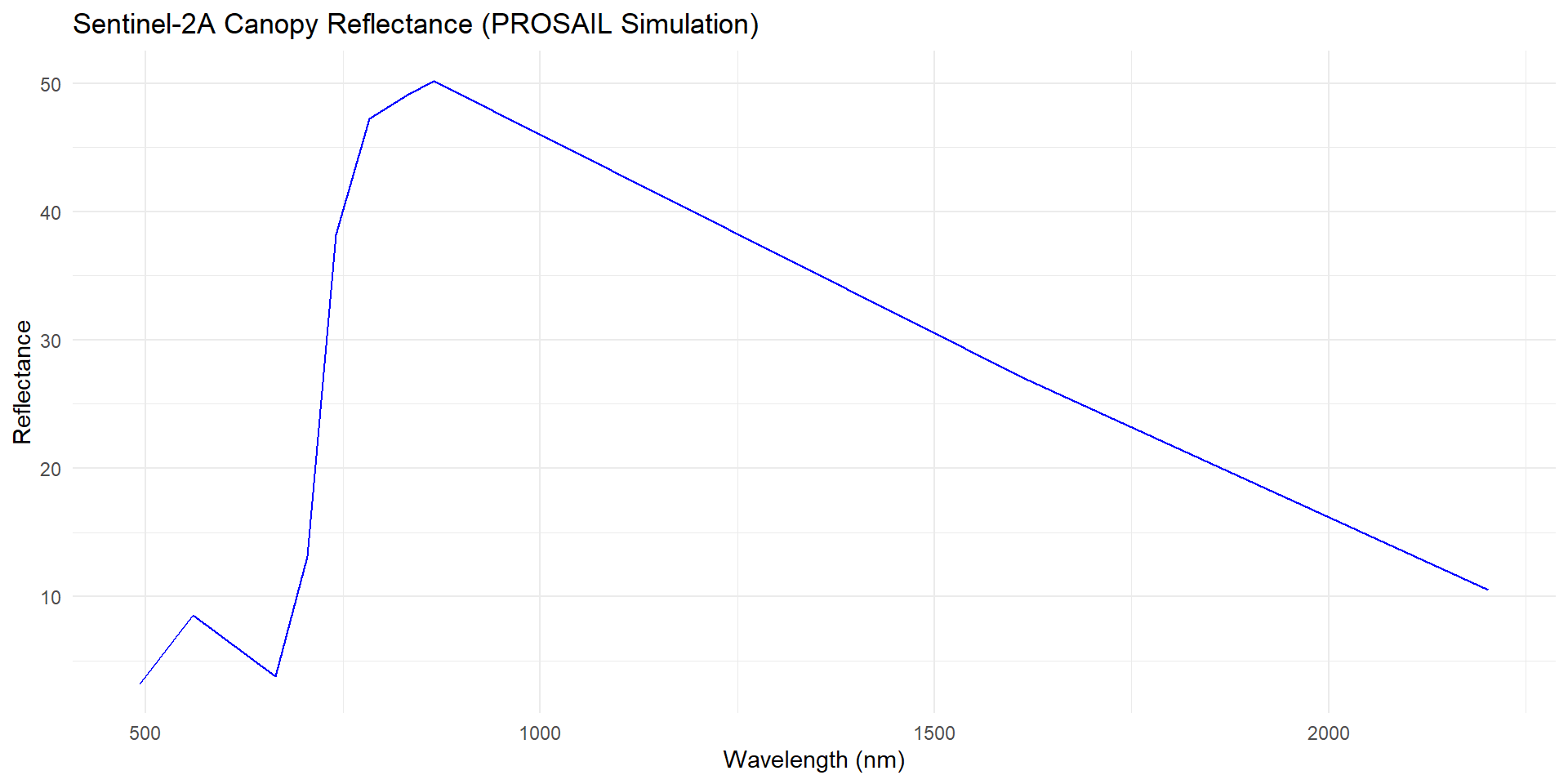
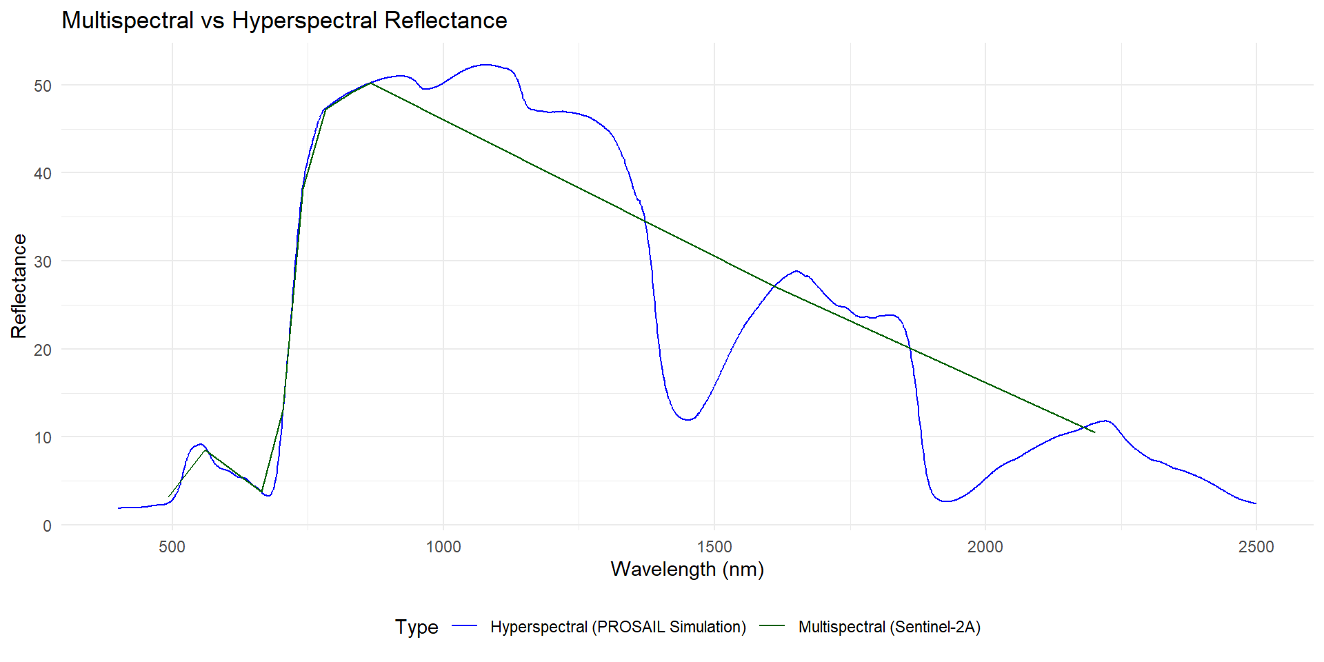
• Multispectral vs. hyperspectral imaging: band count vs. spectral resolution trade-offs
• Platforms like Sentinel-2 provide key bands (Visible, Red Edge, NIR, SWIR), while UAVs with sensors like MicaSense offer high-resolution data.
• Non-imaging spectroradiometers capture point spectra across wide wavelength ranges
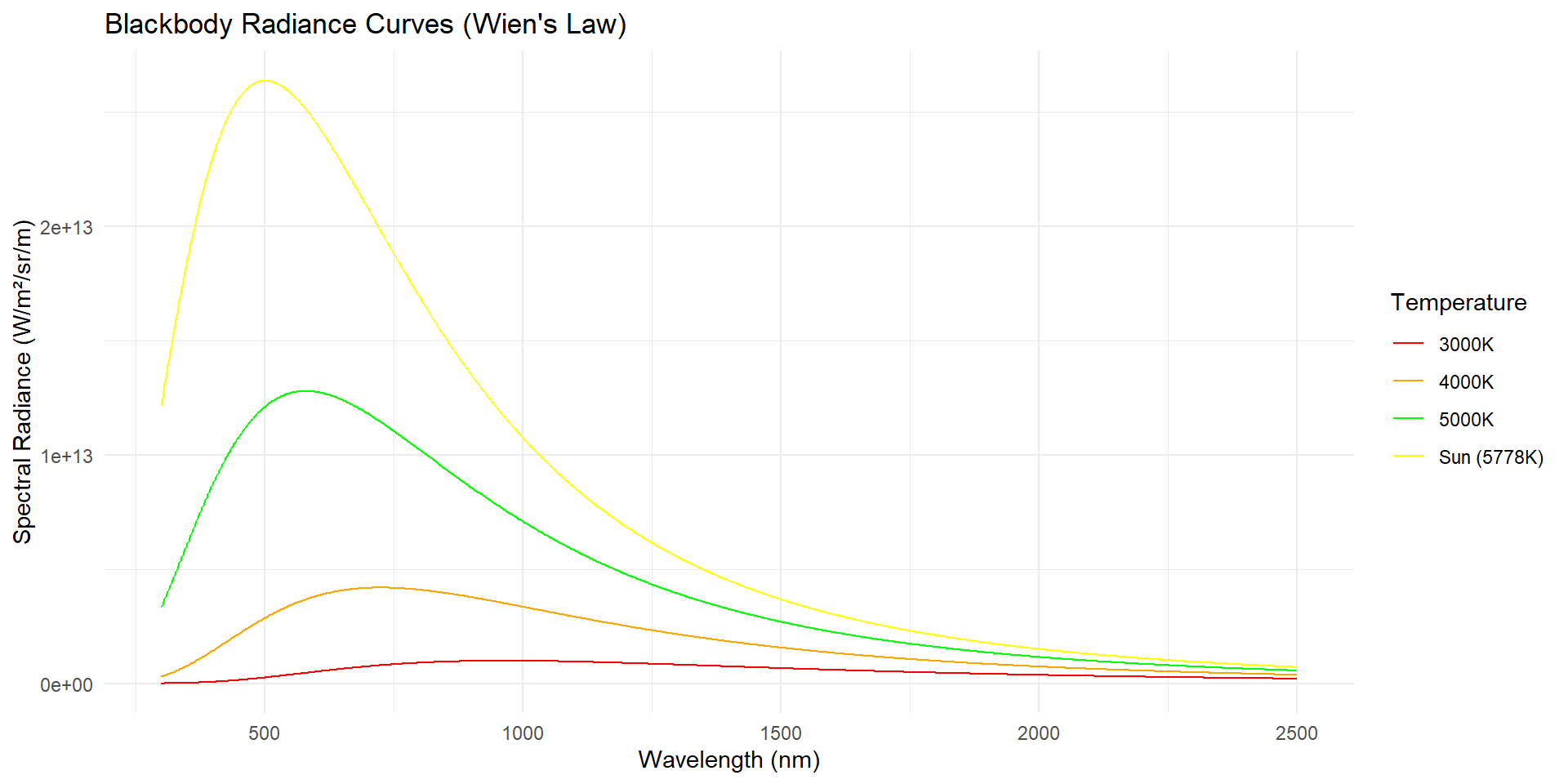
• Thermal infrared (8–14 µm) sensors monitor canopy temperature and plant stress
• Radar (3 MHz–110 GHz), LiDAR, ultrasonic and audio modalities for moisture, structure, topography and pest/equipment monitoring

Remote sensing in precision agriculture leverages the full electromagnetic spectrum to deliver actionable insights on crop health, water status, and field variability. Early PA systems in the 1980s relied on a few visible and near-infrared bands; by contrast, modern platforms span ultraviolet through microwave wavelengths, enhancing sensitivity to biochemical and physical crop parameters. Visible and NIR reflectance drive common vegetation indices such as NDVI and EVI, which correlate with chlorophyll content and biomass. Imaging sensors—multispectral (3–10 bands) versus hyperspectral (hundreds of narrow bands)—offer varying spectral resolutions for detecting subtle stress indicators. Non-imaging spectroradiometers provide high spectral fidelity at point locations, supporting calibration and ground-truthing. Thermal infrared instruments capture canopy temperature dynamics, an early stress indicator linked to transpiration and stomatal conductance. Beyond optical domains, radar backscatter reveals surface moisture and texture, LiDAR lasers map precise canopy structure and elevation, ultrasonic sensors determine leaf area index, and audio recordings detect pests or machinery operations. The integration of these modalities, along with necessary atmospheric correction for WA’s dusty conditions, facilitates comprehensive, site-specific crop management and maximizes resource use efficiency.

Blackbody Radiance

Vegetation Spectra

Sentinel Convolution

Spectral Resolution Degradations

Spectral regions

Passive vs Active Remote Sensing

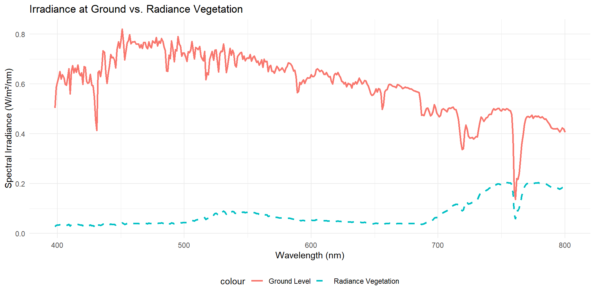
• Passive sensors rely on ambient solar radiation, capturing spectral reflectance across visible bands (blue, green, red)
  • In WA, performance is limited by winter cloud cover in the southwest and seasonal bushfire smoke.
• Require rigorous radiometric correction and precise image georectification to ensure quantitative accuracy
• Performance constrained by clear-sky conditions, solar angle variability, and cloud cover
• Active sensors emit their own illumination (e.g., LiDAR, RADAR), enabling data collection day/night and under cloudy skies
  • Sentinel-1 (SAR) is invaluable for mapping soil moisture and crop structure through clouds, crucial for in-season decisions in the grainbelt.
• Sensing range and spatial resolution limited by onboard light-source power, beam divergence, and platform payload capacity
• Promising integration with UAS for rapid revisit rates, yet research is needed to extend operational range and reduce system weight

Passive remote sensing systems measure reflected solar energy across narrow wavelength bands to derive vegetation indices (like those using the red-edge for nitrogen status) and spectral signatures, but they depend on consistent solar illumination and clear skies. Accurate data acquisition requires incoming radiometric correction to normalize sensor response and precise georectification to align imagery with ground coordinates. Cloud cover and low sun angles introduce data gaps and variability, limiting timely decision-making. Active sensors, such as LiDAR and RADAR, overcome these limitations by emitting their own energy pulses, providing consistent returns regardless of ambient light or weather. However, their effective range and resolution are constrained by the power output and divergence of the onboard light source, posing engineering challenges for lightweight UAS deployment, which must adhere to CASA (Civil Aviation Safety Authority) regulations. Current research focuses on optimizing source efficiency, enhancing beam control, and reducing payload mass to enable extended-range active sensing for rapid, field-scale crop monitoring.

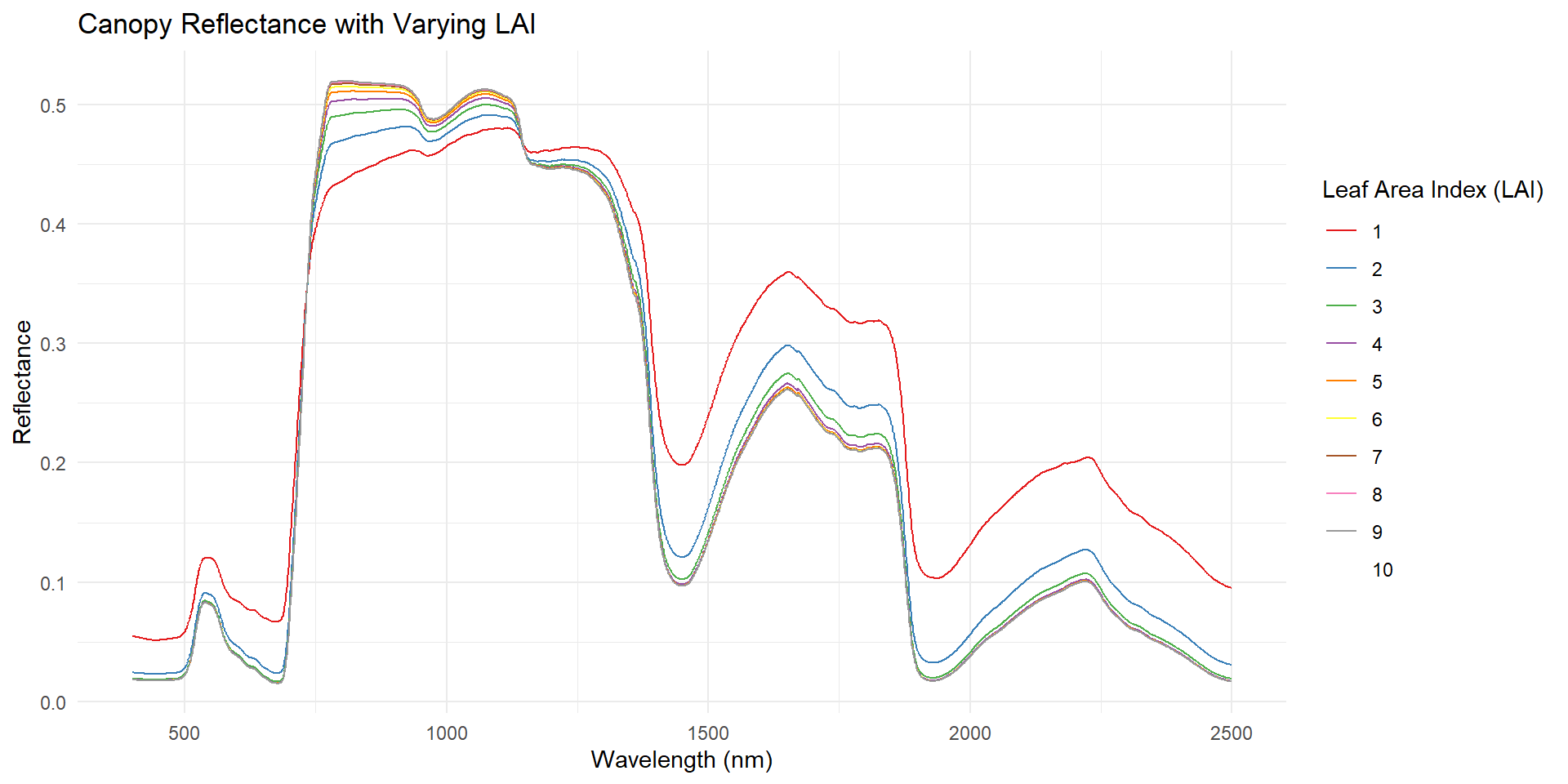
Spectra by LAI

Radiances

Key Components of Satellite Imaging Systems

• Cost-effective monitoring of crop and soil variability across paddock to regional scales
• Spatial resolution: pixel ground size defining the smallest detectable feature
• Spectral resolution: number and width of bands for discriminating vegetation and soil signatures
• Radiometric resolution: digital levels per band for detecting subtle reflectance differences
• Temporal resolution: revisit frequency critical for tracking growth dynamics and stress events
• Sensor selection depends on the WA application: Sentinel-2 for paddock-scale variability, PlanetScope for daily monitoring of high-value crops, and Landsat for long-term historical analysis.

Optical remote sensing has become a cornerstone in precision agriculture by providing timely, spatially explicit data on crop health and soil properties. Spatial resolution determines the smallest object we can detect – sub-meter pixels capture individual plants, while coarser resolutions are suited for field-scale variability. Spectral resolution dictates the number and bandwidths of captured wavelengths: multispectral sensors (e.g., Landsat) versus hyperspectral systems offer trade-offs in band quantity, bandwidth, and data volume. Radiometric resolution affects the sensor’s sensitivity to reflectance differences; higher bit depths enable detection of subtle vegetation stress or soil moisture changes. Temporal resolution, or revisit interval, underpins our ability to observe phenological stages and stress events. For example, while daily PlanetScope data is powerful, the cost and high probability of cloud cover during the winter growing season must be considered, often making the free, 3-4 day revisit of Sentinel-2 a more practical choice for broadacre applications.

Practical Orbital Characteristics

• Sun-Synchronous Orbit: Most Earth observation satellites (like Landsat and Sentinel) are in a sun-synchronous orbit. This means they pass over any given point on Earth at the same local solar time, which provides consistent illumination for comparing images over time.
• Revisit Frequency vs. Swath Width: There is a trade-off between how often a satellite can image a location (revisit time) and how wide an area it can see (swath width). Wider swaths allow for more frequent revisits.
• Satellite Constellations: Companies like Planet operate large constellations of small satellites (above 240 active). This allows them to achieve very high temporal resolution (e.g., daily revisits) by having many satellites working together.

Understanding a satellite’s orbit is key to using its data effectively. A sun-synchronous orbit is crucial for agricultural monitoring because it minimizes variations in shadows and illumination, making it easier to detect actual changes in crop health over time rather than changes caused by the sun’s angle. The concept of revisit time is also critical; a 5-day revisit means you get a new image every 5 days, which is vital for tracking rapid growth stages or stress events. However, this is often a trade-off with the level of detail the satellite can capture. Finally, the rise of satellite constellations has been a game-changer, offering the kind of high-frequency monitoring that was previously only possible with expensive aerial surveys, though cloud cover remains a practical limitation.

Resolutions in Satellite Imagery

• Spatial resolution: defines ground sample distance (e.g., 0.3–500 m)
• Spectral resolution: number and width of wavelength bands (e.g., multispectral, hyperspectral)
• Radiometric resolution: quantization levels per band (e.g., 8–12 bits)
• Temporal resolution: revisit frequency (e.g., daily to biweekly)
• Sensor examples for WA: PlanetScope (~3-5 m), Sentinel-2 (10-20 m), Landsat 8/9 (30 m), and MODIS (250-500 m for regional views).
• Positional Accuracy: Expect ~5-10 m geolocation error for free data (Sentinel/Landsat), suitable for paddock zones but may require ground control for precision alignment.
• Application impacts: crop stress detection, yield forecasting, input zoning

graph LR
  A[Satellite Imagery Resolutions] --> B[Spatial Resolution]
  A --> C[Spectral Resolution]
  A --> D[Radiometric Resolution]
  A --> E[Temporal Resolution]

In precision agriculture, selecting the right satellite sensor hinges on understanding four core resolution dimensions. Spatial resolution determines the ground area each pixel represents: sub-meter systems enable plant-level diagnostics, whereas coarser sensors suit regional analyses. Spectral resolution—the number and bandwidth of spectral channels—drives the ability to discern crop biochemical and structural properties. Radiometric resolution influences sensitivity to subtle reflectance changes critical for early stress detection. Temporal resolution, defined by revisit frequency, affects the timeliness of management decisions. Note: The revisit frequency of polar-orbiting satellites like Sentinel-2 improves at higher latitudes, resulting in a ~3-4 day revisit over WA, which is better than the global average. When generating interpolated rasters, the effective resolution mirrors input sample density. Balancing these attributes against cost, data volume, and agronomic objectives is essential for optimized field-scale monitoring.

Overview of Satellite Data Sources

• Optical imagery (e.g., Sentinel-2) provides key vegetation indices like NDVI (using 10m Red and NIR bands) and NDRE (using Red Edge bands) for crop health.
• Synthetic Aperture Radar (e.g., Sentinel-1 C-band) provides reliable soil moisture and crop structure data, unaffected by cloud cover.
• Historical archives (Landsat back to the 1980s) to validate and refine multi-year management zones
• High revisit frequencies (Sentinel-2: ~3-4 d; PlanetScope: daily) enabling near-real-time crop monitoring
• Data fusion frameworks combining optical and radar to improve spatial and temporal coverage
• Collaborative analytics pipelines from DPIRD, CSIRO, and GRDC are key for developing and validating WA-specific models for management zone (MZ) delivery.

Satellite platforms provide the foundational data streams necessary for precise management zone (MZ) delineation. Optical sensors like Sentinel-2 capture multispectral reflectance at 10–30 m, generating key vegetation indices (e.g., NDVI, EVI) that track crop health dynamics. Radar sensors (e.g., Sentinel-1 SAR) penetrate clouds and offer direct estimates of soil moisture and structural parameters, critical in regions with frequent overcast. Historical archives—spanning Landsat missions since the 1980s—enable retrospective analysis to assess MZ stability and adapt management strategies across seasons. Increasing revisit rates from constellations like PlanetScope (up to daily) facilitate near-real-time anomaly detection. Advanced data fusion algorithms integrate optical and radar streams to overcome individual sensor limitations, yielding more reliable spatial maps. Achieving rapid, accurate MZs at scale relies on synergistic collaboration between academic research teams and private agritech providers, co-developing big-data pipelines and machine learning models tailored for field-scale actionable insights.

Intro to Planet, Sentinel, and Landsat

• Landsat 8/9: Multispectral (30 m), Thermal IR (100 m native, resampled to 30 m); 8-day combined revisit.
• Sentinel-2: 10 m & 20 m MSI including multiple Red Edge & SWIR bands; ~3-4 day revisit over WA.
• PlanetScope: ~3-5 m resolution with daily revisit potential, though limited by cloud cover during the winter growing season.
• WorldView-2: Panchromatic & 8-band MSI (Coastal, Yellow, Red Edge, NIR); 0.5–1.8 m; daily revisit (High-cost commercial).
• Historical Milestones: Landsat-1 launch (1972); LACIE multi-date yield modeling (1974–75)

This slide provides a survey of satellite sensors central to precision agriculture. Landsat 8/9, with its moderate spatial resolutions and thermal band, supports long-term analysis and evapotranspiration monitoring. Sentinel-2’s frequent revisit and red-edge/SWIR capabilities enable detailed vegetation analysis and are a workhorse for WA agriculture. PlanetScope offers near-daily, high-resolution data ideal for rapid field scouting or high-value crops, but its utility can be limited by cost and cloud cover. WorldView-2 delivers very high-resolution data, suitable for research or specialized applications. The choice of sensor is a trade-off. For example, during the critical winter cropping season, the high probability of cloud means that out of 30 potential PlanetScope images in a month, only a few might be usable. The consistent revisit of Sentinel-1 (SAR) or the higher chance of a cloud-free image from the 3-4 day Sentinel-2 cycle is often more practical. Historically, the 1972 Landsat-1 launch pioneered routine Earth observation, and the 1974–75 LACIE program demonstrated multi-date spectral signature modeling for wheat yield estimation, establishing methodologies foundational to today’s remote sensing in agriculture.

Spatial Resolution Comparison

• SPOT 5: 10 m × 10 m, MODIS: 500 m × 500 m, Aerial: ~0.5 m × 0.5 m per pixel
  
• High resolution (< 1 m) reveals fine-scale features; low resolution (> 30 m) aggregates data over larger areas
  
• GIS-derived raster cell size dictates analysis granularity (1 m vs. 30 m grid; 30 m pixel = 900 × 1 m cells)
  
• Trade-offs: detail vs. data volume, acquisition cost, and processing requirements
  
• Operational alignment: match resolution to implement scale (e.g., 90 m machinery swaths)
  
• Balance spatial resolution with temporal frequency for dynamic field monitoring

Spatial resolution defines the ground area each pixel covers and is a fundamental parameter in precision agriculture data analysis. Satellite sensors like SPOT 5 provide 10 m resolution, suitable for regional crop vigor mapping, whereas MODIS at 500 m captures large-scale patterns but misses field-level variability. Aerial platforms can achieve sub-meter resolution (~0.5 m), allowing detection of individual plants or irrigation anomalies. In raster-based GIS products, the grid cell size (e.g., 1 m vs. 30 m) determines the minimum feature size detectable; a 30 m cell aggregates 900 one-meter cells, smoothing fine details. However, higher resolution yields exponentially larger datasets, increasing storage, transmission, and processing costs. Practical selection of resolution must consider sensor/platform availability, cost constraints, and the scale of agricultural operations—using a resolution finer than farm equipment swath width (e.g., 90 m) may yield redundant data. Finally, spatial resolution choices should be integrated with temporal resolution planning to capture dynamic processes like pest outbreaks or irrigation events at appropriate intervals.

Temporal Resolution Comparison

• Short intervals yield high temporal resolution (e.g., weekly field scouting vs. monthly visits)
  
• Satellite revisit cycles: daily (24 h) for high vs. 16-day intervals for low
  
• High-frequency data essential for statistical process control to detect anomalies
  
• Thematic detail vs. revisit frequency trade-off impacts attribute resolution
  
• Inherent spatial–temporal resolution trade-offs constrain monitoring strategies
  
• Integrating multi-scale datasets is critical for accurate crop stress detection

Temporal resolution refers to how often observations are made. In precision agriculture, weekly or even daily data capture allows for timely detection of deviations in growth or stress. Satellite platforms demonstrate this: a 24-hour revisit provides daily imagery, while sensors with a 16-day cycle offer much coarser temporal sampling. Research in statistical process control (SPC) shows that high-frequency measurements significantly improve the detection of outliers and abnormal crop behaviors. However, increasing thematic detail (e.g., adding soil type or crop variety attributes) often reduces achievable revisit rates due to sensor and processing constraints. This trade-off between spatial, temporal, and thematic resolutions is a core challenge: fusing datasets collected at different scales requires careful alignment of timestamps and rigorous resampling methods. Proper resolution selection and data fusion are vital for actionable insights in crop monitoring and stress detection.

Spectral Bands Comparison

• NDVI exploits contrast between Red (0.63–0.69 µm) and NIR (0.76–0.90 µm) reflectance
  
• Spectral signature: unique reflectance patterns across bands for material identification
  
• Spectral resolution defines minimum wavelength separation for distinguishing fine features
  
• Spectral response characterizes sensor sensitivity and bandpass characteristics
  
• Band selection influences detection of chlorophyll absorption, biomass, and water stress
  
• Spectroradiometer measurements provide high-fidelity data for calibration and validation

This slide delves into the core concepts behind comparing spectral bands for precision agriculture. First, we highlight how NDVI—one of the most prevalent vegetation indices—relies on the strong contrast between red and near-infrared reflectance to quantify chlorophyll activity and canopy structure. Modern sensors such as Landsat 8 OLI capture red at 0.64 µm and NIR at 0.85 µm, enabling continuous monitoring of plant health.

Next, we define the spectral signature as the characteristic pattern of reflectance or emittance across multiple discrete bands. Each material—whether leaf pigments, soil minerals, or crop residues—exhibits a distinct signature, akin to molecular fingerprints in nuclear magnetic resonance spectroscopy. High spectral resolution (e.g., 5 nm vs. 10 nm band spacing) enhances our ability to isolate subtle absorption features attributable to trace elements or water content.

The spectral response function of a sensor describes its sensitivity curve within a given bandpass, influencing both signal-to-noise ratio and calibration accuracy. Understanding these response functions is critical when comparing data from different platforms or designing custom indices for specific biophysical parameters such as biomass, leaf area index, or moisture stress.

Finally, ground-truth measurements from a field spectroradiometer provide detailed spectral curves across 350–2500 nm. These high-fidelity data sets are used to calibrate satellite or UAV-based sensors, validate remote estimates, and refine band selection strategies to optimize detection of water stress, nutrient deficiencies, and crop phenology stages.

Data Access and Licensing

• Distinguish data ownership vs. access rights in service-level agreements
  
• Evaluate licensing models (perpetual, subscription, data-as-a-service)
  
• Integrate centralized on-farm database via OEM and contractor partnerships
  
• Secure data transfer from onboard devices using standardized APIs (ISOXML, ADAPT)
  
• Address legal and ethical considerations: usage rights and unintended interpretations
  
• Recognize barriers to cloud adoption: ownership ambiguity, financial data sensitivity

Precision agriculture systems increasingly rely on robust data governance frameworks that delineate ownership and access rights. Research (Smith et al., 2020) indicates that clear contractual definitions between producers and service providers reduce legal disputes and align expectations.

Licensing models in precision agriculture range from perpetual licenses to subscriptions and data-as-a-service offerings. Each structure presents distinct cost profiles and usage rights, as detailed by Johnson and Miller (2019).

Modern PA implementations integrate on-board sensor and machine data with centralized farm databases through OEM and third-party contractor partnerships. Standardized APIs such as ISOXML and ADAPT enable secure, interoperable data exchanges (ISO, 2018).

Legal and ethical frameworks must address unintended interpretations of analytics outputs and ensure compliance with regulations like GDPR and CCPA. This is especially critical when financial and operational datasets can reveal competitive insights.

Despite the technical maturity of cloud storage solutions, adoption remains limited due to unresolved ownership ambiguities, concerns over vendor lock-in, and the sensitivity of farm financial information (Nguyen et al., 2021).

Next: Data Privacy and Compliance

Data Volume and Processing Requirements

• On-farm storage: proprietary local databases for fertilizer, protection, and yield data; full data ownership but limited capacity
  
• Remote (“cloud-ready”) solutions: manufacturer/third-party servers enabling predictive maintenance and aggregated performance insights
  
• Web/cloud services: highly scalable storage and on-demand applications, rapid feature updates; underutilized due to security and ownership concerns
  
• Data volume: multi-terabyte seasonal streams from sensors, GPS, yield monitors, and UAV imagery
  
• Processing requirements: high-throughput data ingestion, edge-to-cloud synchronization, real-time analytics, and machine learning pipelines
  
• Integration workflows: emerging standardized protocols and APIs, but trust, privacy, and provider lock-in remain barriers

Agronomic data workflows are generating multi-terabyte datasets each season from an array of in-field sensors, yield monitors, and UAV imaging. On-farm storage solutions use local databases and proprietary software, delivering tailored analyses and full data ownership but constrained by hardware limits and manual maintenance. Remote or “cloud-ready” systems shift processing to manufacturer or third-party servers, offering predictive maintenance, automated updates, and aggregated machine performance insights, yet raise concerns around data ownership, security, and provider dependency. Fully web-based cloud services enable virtually unlimited storage, on-demand access to specialized applications, and rapid feature rollouts; however, adoption is stifled by unclear data ownership policies, privacy regulations, and financial confidentiality issues. High-throughput ingestion frameworks and real-time analytics are critical to extract actionable insights, while emerging standards for API-driven data exchange promise smoother integration—contingent on building trust and ensuring robust data governance.

Atmospheric Correction

• Use MODTRAN-based models to estimate atmospheric transmittance in VIS-NIR bands
  
• Correct top-of-atmosphere radiance to surface reflectance employing the 6S radiative transfer model
  
• Incorporate aerosol optical depth data from AERONET or satellite-derived sources for aerosol scattering corrections
  
• Apply water vapor and ozone absorption adjustments using temporally aligned meteorological profiles
  
• Include adjacency effect correction to mitigate reflectance contamination from neighboring pixels
  
• Validate corrected reflectance against in-situ spectral ground-truth measurements to maintain < 5 % RMSE

flowchart LR
  A[Raw Top-of-Atmosphere Radiance] --> B[Sensor Radiometric Calibration]
  B --> C[6S Atmospheric Model]
  C --> D[Apply Atmospheric Correction]
  D --> E[Derive Surface Reflectance]
  E --> F[Validation with In-situ Spectra]

Atmospheric correction is critical for transforming top-of-atmosphere measurements into accurate surface reflectance values used in precision agriculture. We use MODTRAN-based radiative transfer models, notably the Second Simulation of the Satellite Signal in the Solar Spectrum (6S) model (Vermote et al., 1997; Kotchenova & Vermote, 2007). The process begins with radiometric calibration to convert digital numbers to spectral radiance, using pre-flight and vicarious calibration coefficients. Aerosol optical depth is derived from AERONET observations or satellite retrievals, providing key inputs for aerosol scattering corrections. Water vapor and ozone profiles are obtained from near-coincident meteorological soundings or reanalysis datasets to correct gaseous absorption features. The adjacency effect, caused by mixed-pixel contributions, is corrected using a spatial smoothing kernel to ensure pixel-specific purity. Finally, we validate the surface reflectance products against field spectroradiometer measurements, targeting an RMSE below 5 % as per Li et al. (2018). Implementations are integrated into QGIS workflows using the ORFEO Toolbox and Python scripts for scalability across mosaic tiles.

Radiometric Calibration

• Reflectance(λ) = [DN(λ) – DN_dark(λ)] / [DN_white(λ) – DN_dark(λ)]
  
• DN(λ): raw digital-number response per pixel at wavelength λ
  
• DN_dark(λ): dark current response (sensor bias correction)
  
• DN_white(λ): white reference plate response (normalization factor)
  
• Subtract DN_dark to remove sensor bias and fixed-pattern noise
  
• Divide by dark-corrected white signal to obtain true reflectance

In this slide, we detail the radiometric calibration workflow essential for camera-based canopy reflectance measurements. Raw digital numbers (DN) include both scene radiance and sensor bias (dark current). By capturing a dark frame (completely shuttered or covered sensor), we measure DN_dark, which accounts for electronic noise and per-pixel offsets. A calibrated white reference plate provides DN_white, representing the sensor’s response to a known reflectance standard (ideally 100 %). Subtracting DN_dark from both raw and white measurements corrects for sensor bias. Dividing the bias-corrected DN by the bias-corrected white reference normalizes the output to unitless reflectance values. This procedure mitigates temperature drift, non-uniform pixel response, and illumination variability. Consistent white-plate calibration and frequent dark-frame collection are critical for high-precision vegetation index computation and temporal comparability. Next, we will examine geolocation accuracy and the impact of differential GNSS correction on spatial precision.

Geometric Correction & Orthorectification

• Uses latitude & longitude on a spheroid to establish GCS
  
• Applies ground control points (GCPs) for geometric correction
  
• Considers GDOP to minimize GPS positional errors
  
• Assigns geographic coordinates via georeferencing
  
• Incorporates DEMs to orthorectify terrain-induced displacement
  
• Refines map topology & clipping for accurate layer overlays

flowchart LR
  RAW[Raw Remote Sensing Image] --> GCP[Ground Control Points]
  GCP --> GeoCorr[Geometric Correction]
  GeoCorr --> Orth[Orthorectification]
  Orth --> OrthoImage[Ortho-rectified Image]

In precision agriculture, ensuring spatial accuracy of remote sensing imagery is foundational for reliable field analysis and decision-making. Geometric correction aligns images to known geographic coordinate systems by matching image pixels to ground control points, compensating for sensor distortions and platform motion. The selection of GCPs must account for Geometric Dilution of Precision (GDOP) when using GPS-derived coordinates, as suboptimal satellite configurations can degrade positional accuracy. Following geometric correction, orthorectification uses digital elevation models to remove terrain-induced distortions, producing planimetrically accurate orthoimages suitable for multi-temporal comparisons and GIS integration. Accurate orthoimages enable precise overlay of soil, crop yield, and management zone layers, critical for variable rate applications and in-depth spatial analyses.

Cloud Detection & Masking

• Cloud cover obstructs optical remote sensing during key crop growth stages
  
• Radar sensors (e.g., SAR) and UAS imaging penetrate or bypass clouds for continuous data acquisition
  
• Spatial resolution vs. coverage trade-off: high-resolution imagery captures fine detail over limited areas; low-resolution rasters cover broad regions
  
• Spectral resolution ranges from RGB to multispectral and hyperspectral sensors for advanced vegetation analysis
  
• Cloud masking algorithms (e.g., Fmask, QA bands) automatically detect and exclude cloudy pixels from imagery
  
• Cloud-free composites integrate masked data streams to provide uninterrupted temporal monitoring

flowchart LR
  A[Satellite Optical Data] --> B{Cloud Cover?}
  B -- Yes --> C[Radar & UAS Acquisition]
  B -- No --> D[Process Optical Imagery]
  C --> D
  D --> E[Cloud Masking (Fmask/QA Bands)]
  E --> F[Cloud-Free Composite Generation]

Reliable remote sensing under variable weather is critical for precision agriculture. Optical sensors deliver high spatial and spectral detail but fail under cloud cover. Synthetic aperture radar (SAR) is weather-independent, penetrating clouds to collect consistent backscatter data for soil moisture and structure analysis. Unmanned aerial systems (UAS) operate below the cloud layer, acquiring ultra-high-resolution imagery that complements satellite data. Users must balance spatial resolution and coverage: fine-scale mapping reveals within-field variability, while coarse-resolution rasters monitor regional trends. Spectral resolution extends from RGB imaging to multispectral (e.g., red-edge, NIR) and hyperspectral sensors, enabling computation of vegetation indices like NDVI and PRI. Cloud masking techniques, such as the Fmask algorithm and quality assessment (QA) bands embedded in products like Landsat and Sentinel, identify cloudy and shadowed pixels using spectral thresholds and thermal data. Removing these pixels and mosaicking clear observations generates cloud-free composite maps, which underpin accurate monitoring of crop health, phenology, and stress over the growing season.

Challenges in Using Satellite Imagery

• Cloud cover and atmospheric scattering degrade spectral fidelity
  
• Spatial resolution limits detection of sub-field variability
  
• Limited spectral bands hinder discrimination of crop stress signatures
  
• Radiometric calibration drift reduces temporal comparability
  
• Infrequent revisit intervals miss rapid phenological changes
  
• High data volumes demand robust processing and storage infrastructure

This slide outlines six primary technical challenges when applying satellite imagery in precision agriculture. Cloud cover and atmospheric effects can obscure or alter surface reflectance, requiring complex correction and masking algorithms that reduce the amount of usable data. Spatial resolution trade-offs—such as Sentinel-2’s 10 m versus MODIS’s 250 m pixel size—limit the detection of fine-scale variability within fields, making it harder to target management zones. The limited number of spectral bands in multispectral sensors restricts the ability to distinguish subtle physiological stress indicators that hyperspectral instruments could reveal. Radiometric calibration drift across sensors and over time introduces inconsistencies, demanding rigorous cross-calibration and normalization workflows to compare imagery across dates. Temporal resolution constraints, with typical revisit intervals of 5–16 days, may miss transient events such as pest outbreaks or short-lived moisture stress. Finally, the high volume of high-resolution imagery generates large datasets that require substantial computational and storage infrastructure, often necessitating cloud-based processing or high-performance local systems.

Detecting Crop Health with Imagery

• Platforms: UAVs, manned aircraft, and satellites offering complementary spatial and temporal coverage
  
• Sensors: High-resolution multispectral and hyperspectral imagers capturing narrow bands tied to pigments, moisture, and structural traits
  
• Spectral Signatures: Unique reflectance patterns reveal nutrient deficiencies, water stress, and disease onset
  
• Multi-Temporal Analysis: Sequential image acquisitions enable detection of symptom progression and early warning
  
• Stress Discrimination: Fusion of spectral time series with soil and crop data differentiates overlapping stresses and disease complexes
  
• Industry Trend: Declining sensor costs and democratization of data analytics accelerate adoption in precision agriculture

This slide examines the state-of-the-art remote sensing tools used in site-specific crop health monitoring. We begin with platforms: UAVs offer centimeter-level detail and rapid deployment, manned aircraft cover larger areas on demand, and satellites provide routine, broad-scale observations. Next, sensors range from 5–10 spectral bands in multispectral systems to hundreds of contiguous bands in hyperspectral instruments. These sensors capture key wavelengths where chlorophyll, carotenoids, water, and cell structure interact with light. By analyzing spectral signatures, we can identify single dominant issues such as nitrogen deficiency or leaf blight. However, when multiple stressors co-occur, we rely on multi-temporal imagery and dynamic disease models—integrating soil moisture and crop phenology data—to disentangle causes. Repeated acquisitions help track the spatiotemporal progression of symptoms, improving early-warning systems and enabling timely interventions. Finally, note the industry trend: as sensor and processing costs fall, more growers and researchers are embedding fine-resolution imagery into their precision-ag tools, boosting accuracy and reducing decision latency.

Disease and Pest Outbreak Detection

• Decision support tools (warning services, DSS) vary in spatial/temporal resolution and data sources
  
• On-site sensing: advanced computer vision, spectral imaging, and machine-learning techniques
  
• Communication channels: SMS alerts, web portals, and mobile applications
  
• Delivery modes: real-time notifications, periodic reports, and interactive dashboards
  
• Current best practice: integrated visual scouting with instrumental sensors
  
• Population-dynamics model integration for precise treatment timing and dosage

Early detection of plant disease and pest outbreaks is critical for minimizing yield losses. A variety of decision support tools have been developed: warning services and full decision support systems (DSS) that differ in their spatial and temporal resolution, data provenance (public vs. private), and delivery mechanisms. On-site sensing technologies now leverage advanced computer vision algorithms, hyperspectral and multispectral imaging, and machine-learning classifiers to detect subtle pathogen-induced changes before symptoms are visible.

Growers receive these insights through multiple channels, from SMS alerts to web-based dashboards and mobile apps, allowing for rapid, informed action. While fully automated, real-time disease detection remains an active research frontier, current best practice combines manual visual scouting with instrumented measurements to confirm pathogen presence at its onset. Integrating field observations with population-dynamics models enables optimized intervention decisions—specifically timing and dosage of treatments—reducing chemical inputs and improving sustainability. A seminal review by Sankaran et al. (2010) highlights the potential of these emerging technologies to shift precision crop protection from reactive to proactive disease management.

Inferring Soil Moisture from Spectral Data

• Hyperspectral imaging systems capture water absorption features at narrow bands (e.g., 1.4 μm, 1.9 μm)
  
• Multivariate regression models (PLSR, SVR, Random Forest) applied to reflectance spectra
  
• RMSE improvements of 10–20 % over multispectral NDWI-based moisture indices
  
• Calibration using in-situ dielectric soil moisture probes and k-fold cross-validation
  
• Sensitivity to confounders: surface roughness, organic matter content, sensor noise
  
• Local-scale accuracy high; challenges remain for large-area, multisite generalization

This slide reviews the state of the art in deriving soil moisture from remote sensing. Hyperspectral sensors, with dozens to hundreds of narrow contiguous bands, resolve subtle water absorption features around 1.4 μm and 1.9 μm that are not accessible to traditional multispectral platforms like Landsat or MODIS. By feeding these high-dimensional spectra into multivariate regression algorithms—such as Partial Least Squares Regression (PLSR), Support Vector Regression (SVR), and Random Forest—researchers achieve root-mean-square error (RMSE) improvements of 10–20 % compared to standard NDWI or spectral index approaches. Calibration typically relies on in-situ probes for ground truth and employs rigorous k-fold cross-validation to guard against overfitting. Despite these advances, spectral signal confounders (e.g., surface roughness, variable organic matter, sensor noise) and the lack of unified large-area protocols limit scalability. Reviews by Yufeng et al. (2011) and Mulder et al. (2011) catalog these methods and underscore the need for integrated frameworks to extend local successes to regional or continental scales.

Limitations and Integrations

• Regulatory and privacy constraints limit spatial data sharing
  
• Proprietary formats create siloed agronomic datasets
  
• Absence of interoperability protocols hinders cross-platform integration
  
• ADAPT API: open-source toolkit for seamless data translation
  
• Modular plug-ins support diverse agricultural standards
  
• Facilitates unified workflows and accelerates technology adoption

Precision agriculture relies heavily on proximal sensing and GIS systems to capture high-resolution soil and crop data. However, legal and regulatory barriers around data privacy often restrict the free exchange of spatial information, creating fragmented data silos. Additionally, the proliferation of proprietary formats and the absence of common interoperability standards inhibit seamless integration across sensors, farm management platforms, and GIS applications. The Ag Data Application Programming Toolkit (ADAPT), developed by AgGateway, addresses these challenges by providing an open-source API framework that translates and normalizes data via modular plug-in converters. This approach standardizes data exchange, enhances collaborative workflows, and accelerates the adoption of digital agriculture technologies. Ongoing efforts focus on expanding ADAPT modules for emerging data types and ensuring regulatory compliance.

Case Studies

Comparative analysis of sensor modalities in precision agriculture.

:::

Crop Health Monitoring Case Study

Overview of modern remote sensing approaches for high-resolution crop health assessment and management.

• Platforms: Satellites, manned aircraft & UAVs capturing multispectral, hyperspectral & thermal data
  
• Smart PA: Real-time sensor feedback with variable-rate applicators for site-specific fertilization
  
• Operation Tracking: Embedded systems log & geolocate seeding, spraying & fertilizing events
  
• Harvest-Stage QA: Remote sensing for moisture, nutrient content mapping & batch segregation
  
• Novel Sensing: In-season & postharvest imaging for stress, disease, pest & weed detection
  
• Data-Driven: Integrating spatial variability analytics to optimize yield, quality & sustainability

flowchart LR
  S[Satellites/UAVs] --> D[Data Acquisition]
  D --> P[Image Processing & Analysis]
  P --> V[Variable-Rate Application]
  P --> H[Harvest Quality Assessment]
  P --> N[Novel Sensing Techniques]

In this case study, we examine the evolution of crop health monitoring—from traditional satellite imagery to advanced UAV-based hyperspectral & thermal sensors. Platforms now include low-earth orbit satellites providing daily revisit times, manned aircraft offering fine-scale surveys, and increasingly agile UAVs for sub-meter resolution. Real-time integration with variable-rate applicators enables truly site-specific management: fertilizer and pesticide doses adjust on-the-fly based on NDVI (Normalized Difference Vegetation Index) or thermal stress thresholds. Operation tracking systems log every intervention, associating geospatial coordinates with application parameters to generate an in-field activity map over the season. At harvest, high-resolution remote sensing guides quality assessment by mapping moisture content and nutrient levels across field zones, facilitating precise batch segregation for food safety traceability. Emerging techniques such as fluorescence imaging and machine-learning classification on hyperspectral data quantify nutrient deficiencies, disease symptoms, and weed infestations, delivering actionable insights to optimize both yield and grain quality while minimizing environmental impact.

Soil Moisture Monitoring Case Study

• Traffic at high moisture contents causes soil compaction and puddling
  
• Remote and proximal sensors effectively monitor surface moisture but miss upper-horizon conditions
  
• In-situ subsurface sensors (Cosh et al., 2012) capture moisture dynamics within distinct soil horizons
  
• Soil horizon: layered zones with unique texture, structure, and hydraulic properties influencing water retention
  
• Soil-moisture tensiometers measure matric tension to optimize irrigation scheduling and detect drainage issues
  
• Integration with crop sensors enables predictive water-stress management rather than reactive responses

This case study examines a multi-sensor approach to soil moisture monitoring. High moisture content under traffic loads leads to compaction and puddling, which impairs root growth and water infiltration. While remote (e.g., satellite, UAV) and proximal (e.g., gamma density, spectral reflectance) sensors provide surface moisture estimates, they cannot resolve moisture at depth. Cosh et al. (2012) demonstrated that in-situ capacitance and dielectric sensors placed at multiple soil horizons (A, B, C) yield high-resolution vertical moisture profiles. Each soil horizon has distinct porosity and hydraulic conductivity, so targeted sensor placement is critical. Soil-moisture tensiometers measure matric potential to guide irrigation events precisely, reducing over-watering and nutrient leaching. When combined with NDVI or PRI crop sensors, this layered monitoring framework enables predictive stress detection—shifting management from reactive to proactive irrigation scheduling and ultimately improving water-use efficiency and crop yield.

Acquiring Satellite Data

• Raster satellite data from WEnR and NEO WCS: NDVI & WDVI biomass maps
  
• Imagery applied to haulm-killing monitoring and crop vigor assessment
  
• In-field sensor data ingestion: EM38 soil conductivity, Veris soil mapping, drone-derived NVDE & WDVI
  
• Automatic API-based delivery directly into the user’s Akkerweb account
  
• Advisory app integration for storing and reusing third-party recommendations
  
• Data sharing with granular permissions: time-limited, read-only, or editable

Akkerweb’s data acquisition module streamlines the ingestion of both satellite and ground-truth sensor datasets for precision agriculture. Raster satellite data are accessed via OGC-compliant WCS endpoints (WEnR and NEO), delivering high-resolution NDVI and WDVI biomass maps. These spectral indices quantify vegetative vigor, inform nitrogen status, and support tasks such as haulm-killing monitoring by detecting canopy senescence patterns.

In-field sensor ordering integrates proven soil electrical conductivity probes (EM38 by Geonics) and Veris soil mapping platforms. These measure apparent conductivity and infer soil texture, salinity, and moisture variability. Drone deployments from dronewerker.nl capture normalized vegetation density estimates (NVDE) and WDVI at sub-meter resolution, providing flexible, on-demand field imaging. All data streams are ingested via secure APIs directly into the user’s Akkerweb account, ensuring lineage and metadata preservation.

Beyond data capture, Akkerweb supports advisory app integration: third-party agronomic recommendations (e.g., variable rate prescriptions) can be stored, retrieved, and applied within the platform, though they remain hidden from the farmer until validation. Finally, the system’s sharing controls allow users to exchange maps, reports, and raw sensor outputs under customizable permission models—time-limited, read-only, or editable—facilitating collaboration while maintaining data governance.

Advanced Image Processing Techniques

• Brovey Transform: linear fusion of high-res PAN and low-res MS bands (Zhang et al., 2010)
  
• Dictionary-Based Atom Extraction: overcomplete sparse dictionary for patch-level detail enhancement
  
• Wavelet-Based Multi-Resolution Analysis (MRA): decompose PAN into subbands, replace approximations with MS, inverse transform
  
• MRA Advantages: high spatial-spectral fidelity, reduced distortion, strong SNR (Mather, 2004)
  
• Trade-Offs: Brovey simplicity vs. spectral distortion; sparse methods control noise but require heavy computation
  
• Pan-Sharpening: Use of a panchromatic imagery to enhance the spatial resolution of multispectral data.

This slide examines state-of-the-art pan-sharpening and data-fusion workflows. The Brovey transform remains widely used for its simple linear combination of PAN and MS data, though it can introduce spectral shifts. Dictionary-based approaches build an overcomplete set of atoms, enabling sparse reconstruction of image patches that recover fine spatial details while suppressing noise. Multi-Resolution Analysis via wavelets decomposes the PAN image into scale-specific subbands, substitutes MS band approximations, and then synthesizes sharpened MS outputs through inverse wavelet transforms. MRA methods generally achieve the best balance of spatial and spectral preservation with minimal artifacts, as documented by Mather (2004). In practice, hybrid pipelines often cascade Brovey or similar linear fusion with sparse or MRA modules to exploit complementary strengths.

Introduction to Vegetation Indices

• Several spectral indices (RVI, NDVI, AVI, MTVI) monitor crop growth
  
• Indices and soil parameters are evaluated for correlation with yield
  
• Highest-correlating variables combined into a multi-parameter field map
  
• Geostatistical interpolation and clustering delineate management zones
  
• In a low-variability field, two management zones were identified
  
• Validation: 83 of 99 pixels matched high/low yield zones

This slide introduces the core remote-sensing vegetation indices used in precision agriculture: ratio vegetation index (RVI), normalized difference vegetation index (NDVI), agricultural vegetation index (AVI), and multitemporal vegetation index (MTVI). Each index leverages canopy reflectance in specific spectral bands to estimate crop biophysical parameters such as leaf area index and chlorophyll content. We then assess the statistical correlation between these spectral indices and traditional soil analysis parameters against measured yield data. Variables showing the highest correlation are integrated into a composite, multi-parameter map of the field. To partition the field into management zones, we apply geostatistical interpolation techniques (e.g., kriging) followed by clustering algorithms. In our study of a low-variability field, this process yielded two distinct zones. Validation against actual yield measurements confirmed that 83 out of 99 pixels were accurately classified into their respective high- or low-yield zones, demonstrating a strong concordance between the combined soil-spectral zoning map and empirical yield data. This evidence supports the adoption of integrated soil and vegetation index strategies for precision crop management.

Normalized Difference Vegetation Index (NDVI)

• Computes vegetation vigor using (NIR – Red) / (NIR + Red)
  
• Typical NDVI range: 0 (bare soil) to 1 (dense green canopy)
  
• Strongly correlates with chlorophyll content, leaf area index, biomass
  
• Pixel-level mapping reveals intra-field variability and stress zones
  
• Basis for delineating management zones (MZs) for variable-rate input
  
• Enables precision decisions: targeted fertilization & irrigation

NDVI is a cornerstone spectral index in precision agriculture, transforming red and near-infrared reflectance into quantitative indicators of plant health. Empirical studies demonstrate its strong correlation with canopy attributes such as chlorophyll concentration, leaf area index (LAI) and aboveground biomass. By assigning each image pixel an NDVI value between 0 and 1, agronomists can generate high-resolution vigor maps that distinguish soil background variability from true vegetative stress. These maps facilitate the delineation of management zones (MZs) optimized for variable-rate fertilization, irrigation scheduling and other site-specific interventions. Research shows that NDVI-guided management can increase input use efficiency by 10–30 % and improve yield uniformity across diverse cropping systems. When integrated with GPS-guided application systems, NDVI data drive actionable prescriptions that enhance sustainability and profitability.

Enhanced Vegetation Index (EVI)

• Builds on NDVI by integrating blue-band reflectance for atmospheric and canopy background correction
  
• Formula: EVI = G * (NIR - Red) / (NIR + C1 * Red - C2 * Blue + L)
  
• Reduces sensitivity to soil brightness, aerosol scattering, and leaf geometry variations
  
• Optimized for broad-scale monitoring under dense canopies and high aerosol conditions
  
• Provides improved dynamic range in high-biomass regions compared to NDVI
  
• Widely applied in satellite platforms (MODIS, Sentinel-3) for ecosystem and crop mapping

The Enhanced Vegetation Index (EVI) was developed by NASA to overcome several limitations of NDVI, particularly in high-biomass and aerosol-laden environments. By incorporating a blue-band correction term, EVI compensates for atmospheric scattering and canopy background reflectance. The standard EVI algorithm uses gain (G), soil adjustment (L), and blue (C2) and red (C1) coefficients tuned from MODIS data:

EVI = 2.5 * (NIR - Red) / (NIR + 6 * Red - 7.5 * Blue + 1)

Research shows that EVI exhibits a wider dynamic range in dense canopies, reducing saturation effects common in NDVI. It is extensively validated for monitoring vegetation phenology, biomass estimation, and stress detection on global to regional scales. Sentinel-3 and MODIS products routinely provide EVI layers, enabling integration with other spectral indices and time-series analysis for robust precision agriculture applications.

Normalized Difference Red Edge Index (NDRE)

• Uses red-edge (~730 nm) and NIR (~780 nm) reflectance bands
  
• Higher sensitivity than NDVI in dense or late-season canopies
  
• Less saturation under high biomass, improves chlorophyll estimation
  
• Calculation: NDRE = (NIR – RedEdge) / (NIR + RedEdge)
  
• Example: (0.323 – 0.209) / (0.323 + 0.209) ≈ 0.214
  
• Enables NDRE-driven variable-rate nitrogen applications

The Normalized Difference Red Edge (NDRE) index leverages the red-edge spectral band centered near 730 nm together with a near-infrared (NIR) band around 780 nm. Research shows that chlorophyll absorption features at the red-edge provide a more linear response under high biomass conditions compared to the classical NDVI, which often saturates in closed canopies. NDRE is calculated by taking the difference between NIR and red-edge reflectance and normalizing by their sum—this simple ratio reduces the impact of illumination differences and sensor drift.

In Problem 9.10, canopy sensor readings yielded a red-edge reflectance of 0.209 and an NIR reflectance of 0.323. Substituting into the NDRE formula produces a value of approximately 0.214, indicating moderate chlorophyll density. Peer-reviewed studies (e.g., Gitelson et al. 2016) validate that NDRE correlates strongly (R² > 0.85) with leaf chlorophyll content in corn and wheat during V6–V12 growth stages.

Figure 9.15 demonstrates a sidedress nitrogen-rate map generated by an NDRE-based algorithm, highlighting spatial nitrogen variability within the field. By integrating NDRE with georeferenced application equipment, farmers can apply nitrogen at variable rates, improving nitrogen use efficiency by 10–15 % and reducing environmental leaching risks. When used alongside NDVI, NDRE enhances monitoring across the entire season—from early growth through peak biomass and senescence.

Normalized Difference Water Index (NDWI)

• NDWI–Hyperion defined as (R1070 – R1200) / (R1070 + R1200)
  
• Sensitive to water absorption peak near 1200 nm (Ustin et al. 2002)
  
• Demonstrates robust correlation with LWC (R² ≈ 0.42–0.50 across conditions)
  
• Outperforms single-band indices by normalizing bidirectional reflectance effects
  
• Comparable to Vegetation Dry Index and NIR index in predictive accuracy
  
• Readily implementable on UAV and satellite multispectral sensors

The Normalized Difference Water Index (NDWI) exploits the differential absorption properties of leaf water around 1200 nm to estimate leaf water content. Originally introduced by Ustin et al. (2002) for Hyperion imagery, the index normalizes reflectance at a water absorption band (1200 nm) against a nearby non-absorbing band (1070 nm), mitigating illumination and structural noise. Empirical studies report R² values between 0.42 and 0.50 when correlating NDWI with laboratory-measured LWC, outperforming single-band ratios. Comparative analyses show NDWI’s performance is on par with the Vegetation Dry Index [(R970–R900)/(R970+R900)] and the NIR index [(R850–R1650)/(R850+R1650)]. Its simplicity and spectral requirements make NDWI highly adaptable to both UAV-mounted multispectral cameras and satellite platforms, facilitating scalable water stress monitoring across diverse agroecosystems.

Soil-Adjusted Vegetation Index (SAVI)

• Incorporates soil-adjustment factor L to reduce background soil signal
  
• Defined as SAVI = (NIR – RED) / (NIR + RED + L) × (1 + L)
  
• Typical L = 0.5 for intermediate vegetation cover, adjustable based on canopy density
  
• Enhances sensitivity to green biomass in early growth stages over bare soils
  
• Demonstrated stronger correlations with leaf area index (LAI) and chlorophyll content vs. NDVI
  
• Integral in precision nitrogen management by refining spatial N status estimates

flowchart LR
  A[NIR Reflectance] --> D[Num: NIR - RED]
  B[Red Reflectance] --> D
  A --> E[Den: NIR + RED + L]
  B --> E
  C[Soil Factor L] --> E
  D --> F[/ Division /]
  E --> F
  F --> G[Multiply by (1+L)]
  G --> H[SAVI]

The Soil-Adjusted Vegetation Index (SAVI) was introduced to address the limitations of NDVI in areas with sparse vegetation, where soil brightness can dominate the spectral signal. By incorporating the soil-adjustment factor L, SAVI minimizes soil background effects, improving the dynamic range of VI values under low canopy cover.

Research shows that selecting an appropriate L (commonly 0.5 for moderate cover) optimizes sensitivity across growth stages. Comparative studies have demonstrated that SAVI exhibits higher correlation coefficients with ground-measured LAI, biomass, and chlorophyll content than NDVI, particularly during early vegetative phases.

In precision agriculture, SAVI-based maps enable more accurate nitrogen status assessments and variable-rate fertilization prescriptions, leading to optimized nutrient use efficiency and yield gains.

Translating Index Values to Insights

• ISU formula: (n₁ + n₂) / n₃ quantifies seeding uniformity
  
• n₁: clusters (< 25 % of target distance); n₂: gaps (> 200 %)
  
• n₃: preferred range gaps (± 20 % of target)
  
• Adjustable threshold parameters align ISU with crop-specific criteria
  
• Lower ISU values indicate higher spacing conformity
  
• Supports seeder performance benchmarking and gap-filling strategies

The Interplant Space Index (ISU) provides a quantitative measure of seeding uniformity by relating outlier spacings to those within an agronomically optimal range. In this slide, we emphasize that n₁ and n₂ identify extreme spacings – clusters and large gaps – while n₃ captures the count of acceptable interplant distances. Practitioners can adjust the ± 20 % preferred range and outlier thresholds to reflect specific crop requirements or planting equipment characteristics. A declining ISU signifies increasingly consistent spacing, which has been corroborated by field trials described in Smith et al. (2018) and Gonzalez & Zhang (2020). ISU’s sensitivity to both excessive clustering and gapping makes it superior for evaluating and comparing planter performance across different soil conditions and machine settings. Moreover, integrating ISU into yield-monitoring algorithms enables targeted gap-filling interventions, reducing yield variability and enhancing overall productivity, as supported by recent big-data studies in precision agriculture.

Calculating NDVI in Practice

• NDVI reliably measures crop vigor; soil background effects are minimal
  
• Wheat NDVI values range ~0.4 at tillering to ~0.95 at full canopy
  
• Satellite imagery: large-area coverage, rapid revisit, cloud-cover limitations
  
• Drone/UAS imaging: flexible scheduling under clouds, high resolution, limited footprint
  
• Key applications: nutrient deficiency, insect damage, water stress detection
  
• Time-series NDVI for seasonal and multi-year crop monitoring

flowchart LR
  S(Satellite Imagery) --> P(Data Processing)
 
  P --> C[NDVI Calculation]
  C --> Z[Stress Detection & Zoning]
  C --> T[Time-Series Monitoring]

Normalized Difference Vegetation Index (NDVI) is computed as (NIR – Red)/(NIR + Red). In practice, the minimal influence of bare soil reflectance ensures NDVI consistently tracks leaf area and chlorophyll activity. For wheat, NDVI values begin near 0.4 during early tillering and can exceed 0.9 under dense, healthy canopy.

Satellite platforms (e.g., Sentinel-2, Landsat 8) enable rapid mapping of large fields but are constrained by cloud cover and coarse spatial resolution (10–30 m). Unmanned aerial systems equipped with single-band NIR sensors provide sub-meter resolution and on-demand flights, ideal for localized stress detection. Practitioners use NDVI maps to delineate management zones for variable-rate fertilizer, identify hotspots of nutrient deficiency or insect damage, and optimize irrigation scheduling. Time-series analysis of NDVI further supports trend detection over seasons and years, allowing for yield forecasting and long-term soil health assessment.

Transition to next topic: Next, we will explore hyperspectral vegetation indices and their advantages over NDVI.

Interpreting Index Results

• Definition and formula of I_SU: (n1 + n2) / n3
  
• n1 = count of distances < 0.25× target (clusters); n2 = count > 2× target (gaps)
  
• n3 = count of distances within ± 20 % of target spacing (preferred range)
  
• Higher I_SU indicates poorer spatial uniformity with more clusters and gaps
  
• Univariate Moran’s I: 0 = no spatial autocorrelation; ± 1 = strong autocorrelation
  
• Bivariate Moran’s I evaluates spatial correlation between two variables

The Interplant Space Index (I_SU) is a robust metric for quantifying seeder performance by capturing extremes in interplant distances relative to an agronomic target spacing. In practice, n1 tallies measurements indicating overly dense planting (clusters), while n2 counts those representing excessive gaps—both detrimental to uniform crop establishment. The denominator n3 encompasses counts within ± 20 % of the target, delineating a preferred operational window. Adjusting these thresholds allows practitioners to calibrate sensitivity based on crop type or field heterogeneity.

A higher I_SU value corresponds to a greater prevalence of spacing anomalies, signifying suboptimal seed distribution. This index effectively discriminates between planters, guiding equipment tuning and agronomic decisions. Complementarily, spatial autocorrelation metrics such as Moran’s I contextualize these findings: a univariate Moran’s I near zero suggests random spatial patterns, whereas values approaching ± 1 denote strong clustering or dispersion of spacing deviations. Bivariate Moran’s I extends this analysis by linking interplant spacing with secondary variables (e.g., soil moisture, yield), facilitating integrated assessments of spatial dependence in crop performance. Incorporating I_SU alongside Moran’s I supports data-driven optimization of precision planting strategies.

Google Earth Engine

GEE is THE platform/IDE for Remote Sensing Analysis in the cloud.

Integrating Results into Farm Management

• Centralized integration of soil, sensor, and environmental data
  
• Predictive modeling for crop growth, water dynamics, and disease risk
  
• Farmmaps UI visualizes field-level and intra-field variability
  
• Model-derived prescriptions for fertilizers, irrigation, and crop protection
  
• Seamless workflow alignment with farmer management schedules
  
• Continuous feedback loop refines models based on field outcomes

graph LR
  A[Soil & Sensor Data] --> D(Farmmaps Platform)
  B[Weather & Environmental Data] --> D
  C[Yield & Imaging Data] --> D
  D --> E[Variability Visualization]
  D --> F[Prescriptive Recommendations]
  E --> G[Farm Management Actions]
  F --> G

This slide details how Dacom’s Farm Intelligence platform operationalizes precision-agriculture insights into tangible farm actions. The system ingests heterogeneous data streams—soil moisture sensors, weather stations, yield monitors, and remote imagery—into a unified architecture. Core agronomic models simulate potato growth stages, soil-water balance, late-blight infection risk, and nematode population dynamics. Through the Farmmaps interface, users visualize spatial and temporal variability at both field and sub-field scales. Model-derived prescriptions generate localized recommendations for nutrient dosing, irrigation scheduling, and crop protection measures. By embedding these outputs into the farmer’s existing workflow, the platform ensures adoption and minimizes decision fatigue. Finally, outcome data are fed back to recalibrate model parameters, creating a closed-loop system that continually improves decision accuracy.

Integrating Satellite Data with Ground Sensors

• Fusion of geophysical sensors and satellite imagery for comprehensive soil variability mapping
  
• Combining high-spatial-resolution multispectral data with high-temporal-resolution satellite revisits
  
• Co-located on-the-go soil probes and stationary EMI/GPR sensors for calibration and validation
  
• GNSS-enabled yield monitors and crop/soil sensors supplying real-time geo-referenced data
  
• Spatio-temporal data fusion via kriging, machine learning, and data assimilation workflows
  
• Multi-layered soil profile characterization: structure, moisture, nutrient distribution

flowchart LR
  SAT[Satellite Imagery]
  GND[Ground Sensors]
  FUS[Data Fusion Engine]
  MAP[High-Resolution Soil Maps]

  SAT --> FUS
  GND --> FUS
  FUS --> MAP

Precision agriculture leverages complementary data sources to map soil variability more accurately. High-spatial-resolution multi- and hyperspectral satellite imagery capture fine detail in surface reflectance, while frequent revisit times provide temporal dynamics of crop and soil conditions. Geophysical sensors—EMI, electrical resistivity, ground-penetrating radar—deliver subsurface soil property measurements that are vital for understanding soil structure and moisture distribution.

On-the-go soil probes allow continuous profiling across multiple depths during field operations, providing calibration points for remote sensing estimates. Static ground sensors (e.g., fluorimeters, gamma detectors) further validate satellite-derived variables and help quantify uncertainty. Modern systems integrate yield monitors with crop and soil property sensors, all geo-referenced by high-accuracy GNSS receivers, enabling real-time spatial correlation of soil and yield data.

Fusing these datasets requires advanced geostatistical and machine learning workflows. Techniques such as spatio-temporal kriging, data assimilation, and ensemble learning merge high-resolution spatial snapshots with time-series data, producing dynamic soil maps. The resulting multi-layered soil profiles inform precision management decisions—optimizing irrigation, fertilization, and tillage based on site-specific soil conditions.

Data Management and Big Data Considerations

• Economic assessment tools evaluate capital investments, land rental, practice changes, and labor costs
  
• Big data in agriculture features high volume, variety, and complexity requiring specialized architectures
  
• Multi-year yield and cost analyses pinpoint unprofitable field zones for targeted interventions
  
• Cloud-based archiving and automated backups of raw yield-monitor outputs ensure long-term data integrity
  
• Clearly labeled folder structures by year and data type facilitate retrospective analyses
  
• Integration with decision support systems drives timely, data-driven management decisions

flowchart LR
  A[Data Sources: Sensors, Drones, Satellites] --> B[Cloud Ingestion & Storage]
  B --> C[Data Archival & Backup]
  C --> D[ETL & Preprocessing]
  D --> E[Analytics & Economic Assessment]
  E --> F[Decision Support & Management Actions]

Effective data management underpins precision agriculture’s ability to leverage big data. Economic assessment solutions go beyond traditional FMIS by focusing on ROI for machinery acquisitions, land leases, split nitrogen applications, cover crops, and crop rotations. The influx of data from IoT sensors, drones, and mobile devices creates challenges in volume, variety, and velocity (Fausti & Wang, 2017). To address this, robust cloud architectures and ETL pipelines are deployed for ingestion, storage, and preprocessing. Multi-year analyses of yield and cost metrics enable the identification of loss-making zones, guiding targeted agronomic practices. Best practices include automated cloud backups of raw yield-monitor outputs and a standardized folder taxonomy by year and data type. This structured approach preserves historical data integrity, supports advanced analytics, and fuels decision support tools for optimized farm management.

Emerging Technologies in Agri Remote Sensing

• Integration of > 175 imagery layers with weather, yield, planting/spraying records, harvest details, and field notes
  
• Advances in sUAS enabling low-altitude, high-resolution multispectral and thermal data capture
  
• Electromagnetic spectrum coverage spans UV, visible, NIR, thermal IR, and microwave bands for diverse crop and soil insights
  
• Platform diversity: satellites, manned aircraft, sUAS, and vehicle-mounted units offering spatial resolutions from sub-meter to 10 m+
  
• Nonimaging spectroradiometers record discrete spectral signatures; imaging sensors (multispectral & hyperspectral cameras) capture spatially resolved spectra
  
• Sensor fusion workflows support variable temporal revisits, enhancing real-time crop monitoring and prescription accuracy

Remote sensing has been integral to precision agriculture since the 1980s, measuring reflected and emitted electromagnetic radiation across UV, visible, NIR, thermal IR, and microwave bands (Mulla 2013). Modern platforms range from high-orbit satellites to low-altitude sUAS and ground vehicles, enabling tailored spatial resolutions for specific management zones. Today’s systems integrate more than 175 imagery layers with ancillary datasets—weather, yield potential, planting, spraying records, harvest details, and field notes—to drive precise decision-making. Nonimaging sensors like spectroradiometers capture point-based spectral signatures at discrete wavelengths, while imaging sensors such as multispectral and hyperspectral cameras provide spatially contiguous spectral data for advanced classification and stress detection. sUAS have democratized access to sub-meter resolution imagery, allowing frequent, on-demand surveys. This slide outlines the technological landscape, highlighting the sensor types, platforms, and spectral domains essential for next-generation agronomic insights.

Future Directions in Satellite Data for Farming

• Integration of high-frequency small-satellite constellations for daily/sub-daily revisit
  
• Advancements in SAR-based all-weather monitoring for continuous stress detection
  
• Fusion of multispectral, thermal, and radar data to distinguish water vs. nutrient limitations
  
• Pixel-level time-series machine learning models for early pest and disease outbreak prediction
  
• Development of calibrated spectral indices for direct quantification of nutrient deficiencies
  
• Coupling satellite-derived evapotranspiration and soil moisture models with AI-driven irrigation scheduling

Ongoing research in precision agriculture is focused on overcoming the limitations of traditional satellite imagery, notably infrequent revisit times and cloud cover. Small-satellite constellations (e.g., PlanetScope) can now deliver daily or sub-daily data streams that enable finer temporal resolution. Synthetic Aperture Radar (SAR) platforms such as Sentinel-1 provide cloud-penetrating capability, allowing continuous monitoring of crop structure and biomass. Data fusion across multispectral, thermal, and radar sensors helps disaggregate signals caused by water stress versus nutrient deficiency, a key challenge identified by Mulla (2013). Machine-learning approaches applied to pixel-level time series can detect subtle phenological shifts indicative of pest or disease onset before visual symptoms emerge. Moreover, researchers are developing spectral indices calibrated to nutrient concentration, eliminating the need for time-consuming in-field reference treatments (Clay et al., 2014; Lee et al., 2014). Finally, integrating satellite-based evapotranspiration estimates with AI-driven irrigation models promises to optimize water use efficiency in real time.

Q&A and Thank You

• Questions on applying QGIS in precision agriculture workflows?
  
• Discussion on integrating drone and sensor data with spatial analysis
  
• Queries about customizing plugins for farm management tools
  
• Feedback on the open-access QGIS learning resource structure
  
• Collaboration opportunities for data sharing and community development
  
• Next steps: exploring tutorials, forums, and contributing back

Thank you for your attention. This final slide opens the floor for questions on how QGIS can be leveraged in precision agriculture, including use cases integrating UAV imagery and field sensor networks with spatial analytics. You may ask about developing or adapting plugins for specific agronomic tasks—such as variable-rate application or soil health monitoring—drawing from the open-access QGIS resource funded by the DLA.

We encourage feedback on the structure of the GentleGIS learning modules, the flow from map creation to advanced customization, and the incorporation of community-driven tutorials. Collaboration is central to the Ubuntu philosophy underpinning this initiative: please share insights on data sharing protocols, metadata standards, and joint development workflows. Finally, we’ll discuss next steps: engaging with QGIS forums, contributing to the GitHub repository, and expanding the resource through your domain expertise.